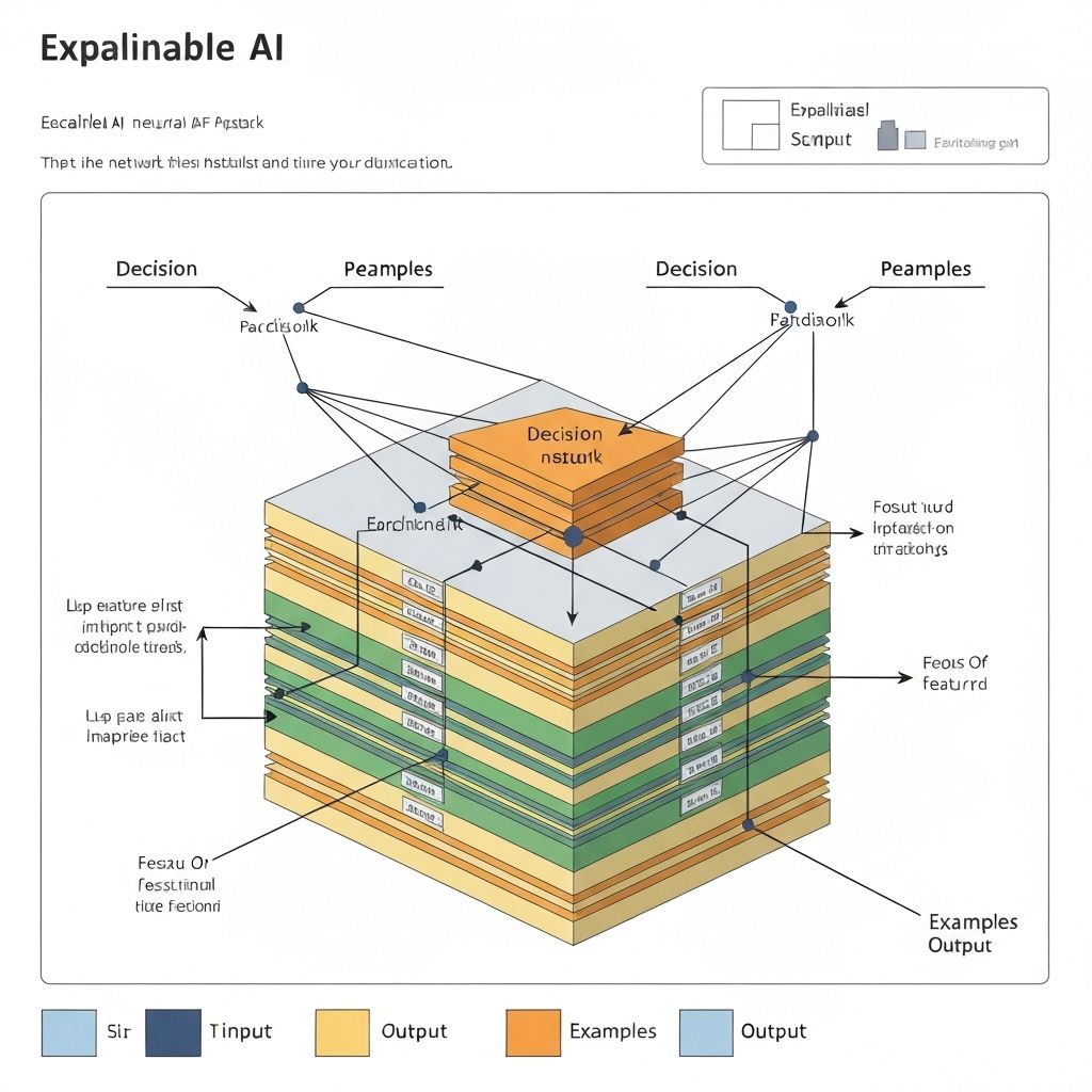
The Rise of Explainable AI (XAI): Opening the Black Box

Section 1: Mathematical Foundations of Model Interpretability

Modern deep learning architectures prioritize minimizing empirical risk over input feature attribution. Consider a neural network model \x24f: \mathbb{R}^d \to \mathbb{Y}\x24 parameterized by \x24\theta \in \Theta\x24. For a given classification task, the model output represents a probability distribution over class labels. The decision boundary constructed by \x24f(x)\x24 is highly non-linear due to the composition of multiple activation layers:

\x24\x24f(x) = \sigma(W_L \cdot \sigma(W_{L-1} \cdot \dots \sigma(W_1 x + b_1) \dots + b_{L-1}) + b_L)\x24\x24

Because the dimensionality \x24d\x24 is typically large (\x24d \gg 10^3\x24) and the number of layers \x24L\x24 introduces non-convex mappings, directly tracing the contribution of an individual feature \x24x_i\x24 to the output \x24f(x)\x24 is analytically intractable. This opacity is the core limitation of black-box models.

To formalize explainability, we define an explanation model \x24g \in G\x24, where \x24G\x24 is a class of interpretable models (e.g., sparse linear models or decision trees of depth \x24D \le 3\x24). The local explanation for a specific prediction \x24f(x)\x24 is defined under a proximity measure \x24\pi_x(z)\x24, which defines the neighborhood around \x24x\x24. We formulate the explanation optimization problem as:

\x24\x24\xi(x) = \arg\min_{g \in G} \mathcal{L}(f, g, \pi_x) + \Omega(g)\x24\x24

Where \x24\mathcal{L}\x24 represents the fidelity loss measuring how close the surrogate model \x24g\x24 is to the black-box model \x24f\x24 within the locality defined by \x24\pi_x\x24, and \x24\Omega(g)\x24 represents the complexity penalty of the explanation model (e.g., the number of non-zero weights in a linear model or the leaf count of a decision tree).

Section 2: Global vs. Local Interpretability

Interpretability methods are broadly categorized along two dimensions: intrinsic vs. post-hoc, and local vs. global.

• Intrinsic Interpretability: Design-level transparency where the model's structural configuration permits direct validation (e.g., Gen\x65ralized Additive Models (GAMs), shallow decision trees, sparse linear models).
• Post-hoc Interpretability: Methods applied to extract explanations from a trained black-box model (e.g., LIME, SHAP, Integrated Gradients).
• Local Explainability: Explaining why the model made a specific prediction for a single instance \x24x\x24.
• Global Explainability: Describing the ov\x65rall behavior of the model across the entire dataset \x24\mathcal{D}\x24. This involves computing aggregate feature importance, global decision rules, or main effects.

Under global explainability, we calculate the av\x65rage attribution of feature \x24i\x24 across all samples in a dataset of size \x24M\x24:

\x24\x24\text{Global Attribution}i = \frac{1}{M} \sum{j=1}^M |\phi_i(x^{(j)})|\x24\x24

This provides a macro-view of features influencing model execution. However, global summaries can obscure localized sub-population behavior, where a feature might have high positive attribution for one subgroup and high negative attribution for another.

Section 3: Local Interpretable Model-Agnostic Explanations (LIME)

The LIME framework computes local attribution by perturbing the target instance \x24x\x24 and learning a sparse linear surrogate model on the gen\x65rated perturbations.

\x60\x60\x60python import numpy as np from sklearn.linear_model import Ridge from sklearn.metrics import r2_score

class LocalSurrogateLIME: def init(self, kernel_width=0.25, num_perturbations=1000): self.kernel_width = kernel_width self.num_perturbations = num_perturbations

def _compute_rbf_kernel(self, distances):
    return np.exp(- (distances ** 2) / (self.kernel_width ** 2))

def explain_instance(self, instance, predict_fn, feature_names=None):
    num_features = len(instance)
    # Gen\x65rate perturbations in the neighborhood of the instance
    perturbations = np.random.normal(0, 1, size=(self.num_perturbations, num_features))
    perturbed_data = instance + perturbations
    
    # Get target predictions from the black-box model
    y_perturbed = predict_fn(perturbed_data)
    
    # If classifier, explain the first class or the predicted class
    if len(y_perturbed.shape) > 1:
        y_perturbed = y_perturbed[:, 0]
        
    # Calculate Euclidean distances and local weights
    distances = np.linalg.norm(perturbed_data - instance, axis=1)
    weights = self._compute_rbf_kernel(distances)
    
    # Fit local weighted ridge regression surrogate model
    local_model = Ridge(alpha=1.0)
    local_model.fit(perturbed_data, y_perturbed, sample_weight=weights)
    
    # Calculate surrogate fidelity (R2 score)
    predictions_surrogate = local_model.predict(perturbed_data)
    fidelity = r2_score(y_perturbed, predictions_surrogate, sample_weight=weights)
    
    explanations = {}
    names = feature_names if feature_names else [f"feature_{i}" for i in range(num_features)]
    for name, coef in zip(names, local_model.coef_):
        explanations[name] = coef
        
    return explanations, fidelity

\x60\x60\x60

The mathematical formulation of the distance weighting kernel is an RBF (Radial Basis Function) kernel:

\x24\x24\pi_x(z) = \exp\left( -\frac{D(x, z)^2}{\sigma^2} \right)\x24\x24

where \x24D(x, z)\x24 is the distance metric (typically Euclidean distance) and \x24\sigma\x24 is the kernel width. LIME assumes that any complex decision boundary is locally linear. However, this assumption breaks down if the kernel width is too large or if the decision boundary is highly disjointed locally.

Vuln\x65rabilities of LIME to Adversarial Manipulation

Research has shown that LIME is highly sensitive to the distribution of out-of-distribution (OOD) perturbed points. An adversary can construct a "scaffolding" wrapper around a biased model: when evaluated on true data inputs, the model behaves biasedly; when evaluated on perturbed inputs gen\x65rated by LIME (which fall outside the true data distribution), the model switches to a fair, unbiased surrogate model. Consequently, LIME will erroneously report that the model is unbiased. This represents a significant security risk for compliance audits.

Section 4: Shapley Additive Explanations (SHAP)

SHAP constructs local feature attributions based on classical coop\x65rative game theory. Features are modeled as players in a coalition, and the prediction is the total payout. The Shapley value \x24\phi_i\x24 of feature \x24i\x24 is the weighted av\x65rage of its marginal contributions across all possible feature subsets:

\x24\x24\phi_i(v) = \sum_{S \subseteq N \setminus {i}} \frac{|S|!(|N| - |S| - 1)!}{|N|!} \left[ v(S \cup {i}) - v(S) \right]\x24\x24

Here, \x24N\x24 is the set of all features, \x24S\x24 is a subset of features excluding \x24i\x24, and \x24v(S)\x24 is the characteristic function representing the expected output of the model when only the features in \x24S\x24 are known:

\x24\x24v(S) = \mathbb{E}[f(X) \mid X_S = x_S]\x24\x24

The Core SHAP Axioms

SHAP is uniquely characterized by satisfying four axiomatic properties:

1. Efficiency (Additive Feature Attribution): The sum of the attributions of all features equals the difference between the model's prediction \x24f(x)\x24 and the baseline expected value \x24\mathbb{E}[f(X)]\x24: \x24\x24\sum_{i \in N} \phi_i(x) = f(x) - \phi_0\x24\x24
2. Symmetry: If two features \x24i\x24 and \x24j\x24 contribute identically to all possible coalitions, their attributions must be equal: \x24\x24\text{If } v(S \cup {i}) = v(S \cup {j}) \text{ for all } S \subseteq N \setminus {i, j}, \text{ then } \phi_i = \phi_j\x24\x24
3. Dummy Player (Null Effect): If a feature \x24i\x24 never changes the model output for any coalition, its attribution is zero: \x24\x24\text{If } v(S \cup {i}) = v(S) \text{ for all } S \subseteq N \setminus {i}, \text{ then } \phi_i = 0\x24\x24
4. Consistency (Monotonicity): If a model changes such that the marginal contribution of feature \x24i\x24 increases or stays the same for all coalitions, its attribution must not decrease: \x24\x24\text{If } v'(S \cup {i}) - v'(S) \ge v(S \cup {i}) - v(S) \text{ for all } S, \text{ then } \phi_i(v') \ge \phi_i(v)\x24\x24

Exact Calculation Complexity

The exact calculation of Shapley values requires evaluating the model \x242^{|N|}\x24 times, which is computationally prohibitive for high-dimensional feature spaces. When \x24|N| = 100\x24, calculating \x24\phi_i\x24 requires \x242^{100} \approx 1.26 \times 10^{30}\x24 model evaluations.

To overcome this, KernelSHAP uses weighted linear regression to approximate the Shapley values, while TreeSHAP exploits the structural properties of tree-based ensembles (such as XGBoost or LightGBM) to optimize the computation time from \x24O(TL2^M)\x24 to \x24O(TLD^2)\x24, where \x24T\x24 is the number of trees, \x24L\x24 is the maximum number of leaves, \x24M\x24 is the number of features, and \x24D\x24 is the maximum tree depth.

\x60\x60\x60python import xgboost as xgb import shap

def train_and_explain_xgboost(X_train, y_train, X_explain): # Train the black-box model dtrain = xgb.DMatrix(X_train, label=y_train) params = { 'max_depth': 6, 'eta': 0.1, 'objective': 'reg:squarederror', 'eval_metric': 'rmse' } bst = xgb.train(params, dtrain, num_boost_round=100)

# Initialize the TreeSHAP explainer
explainer = shap.TreeExplainer(bst)

# Calculate SHAP values
shap_values = explainer.shap_values(X_explain)

# Verify additivity property: base_value + sum(shap_values) = prediction
base_value = explainer.expected_value
predictions = bst.predict(xgb.DMatrix(X_explain))

for idx in range(len(X_explain)):
    sum_shap = np.sum(shap_values[idx])
    assert np.isclose(base_value + sum_shap, predictions[idx], atol=1e-5)
    
return shap_values, base_value

\x60\x60\x60

Section 5: Integrated Gradients for Deep Neural Networks

For deep neural networks, perturbation-based explainers like LIME and SHAP are computationally inefficient. Gradient-based attribution methods compute gradients of the output with respect to the input features. However, simple gradients violate the axiom of Completeness and Implementation Invariance.

Integrated Gradients Axioms

1. Completeness: The attributions of the features sum up to the difference between the model output for the input \x24x\x24 and the baseline \x24x'\x24: \x24\x24\sum_{i=1}^d \text{IG}_i(x) = F(x) - F(x')\x24\x24
2. Implementation Invariance: If two networks are functionally identical (meaning they produce identical outputs for all inputs), their attributions are identical, regardless of the implementation details of the network. Simple gradients or backpropagation heuristics like guided backprop fail this axiom.

Integrated Gradients (IG) resolves these issues by path-integrating the gradients along a straight line from a baseline reference input \x24x'\x24 to the input \x24x\x24:

\x24\x24\text{IG}_i(x) = (x_i - x'i) \times \int{0}^{1} \frac{\partial F(x' + \alpha(x - x'))}{\partial x_i} d\alpha\x24\x24

We approximate the path integral using a Riemann sum across \x24m\x24 steps:

\x24\x24\text{IG}_i^{\text{approx}}(x) = (x_i - x'i) \times \frac{1}{m} \sum{k=1}^m \frac{\partial F\left(x' + \frac{k}{m}(x - x')\right)}{\partial x_i}\x24\x24

Here is a PyTorch implementation of the Integrated Gradients attribution method:

\x60\x60\x60python import torch

class PyTorchIntegratedGradients: def init(self, model): self.model = model self.model.eval()

def compute_attribution(self, input_tensor, baseline_tensor, target_class, steps=50):
    # Ensure gradients are tracked
    input_tensor.requires_grad_()
    
    # Gen\x65rate scaled inputs along the path
    scaled_inputs = []
    for i in range(steps + 1):
        alpha = i / float(steps)
        scaled_input = baseline_tensor + alpha * (input_tensor - baseline_tensor)
        scaled_inputs.append(scaled_input)
        
    scaled_inputs = torch.cat(scaled_inputs, dim=0)
    scaled_inputs.requires_grad_()
    
    # Forward pass through the network
    outputs = self.model(scaled_inputs)
    score = outputs[:, target_class]
    
    # Compute gradients with respect to all scaled inputs
    score.backward(torch.ones_like(score))
    gradients = scaled_inputs.grad
    
    # Av\x65rage the gradients across all steps (excluding the baseline itself)
    avg_gradients = torch.mean(gradients[1:], dim=0)
    
    # Calculate final attribution via element-wise multiplication
    attributions = (input_tensor - baseline_tensor) * avg_gradients
    return attributions.detach().numpy()

\x60\x60\x60

Section 6: Explainable AI in Computer Vision - Grad-CAM

For convolutional architectures, localizing which regions of an image contributed to a classification decision is a primary explanation vector. Gradient-weighted Class Activation Mapping (Grad-CAM) uses the gradients of any target concept flowing into the final convolutional layer to produce a coarse localization map highlighting the important regions in the image.

The saliency map \x24L^c_{\text{Grad-CAM}}\x24 for class \x24c\x24 is computed by taking the weighted sum of the feature map activations \x24A^k\x24 of the final convolutional layer:

\x24\x24L^c_{\text{Grad-CAM}} = \text{ReLU}\left(\sum_k \alpha_k^c A^k\right)\x24\x24

where the weight coefficient \x24\alpha_k^c\x24 represents the importance of feature map \x24k\x24 for class \x24c\x24:

\x24\x24\alpha_k^c = \frac{1}{Z} \sum_i \sum_j \frac{\partial Y^c}{\partial A^k_{i,j}}\x24\x24

Here, \x24Z\x24 is the width times the height of the feature map, and \x24Y^c\x24 is the raw model score for class \x24c\x24 before the softmax activation. The ReLU activation is applied to select only the features that have a positive influence on the class of interest.

Section 7: Counterfactual Explanations

Counterfactual explanations provide actionability by answering: "What is the minimum modification required to the input vector \x24x\x24 to change the model's prediction from \x24y\x24 to a target outcome \x24y^\x24?"* This is mathematically formulated as an optimization problem:

\x24\x24x^* = \arg\min_{x'} d(x, x') + \lambda (f(x') - y^*)^2\x24\x24

where \x24d(x, x')\x24 is a distance metric (e.g., elastic net distance combining Manhattan and Euclidean distances to encourage sparse, small changes), and \x24\lambda\x24 balances the distance minimization against the likelihood of the counterfactual reaching the target prediction.

To make counterfactuals useful in practice, we must enforce physical constraints:

• Immutability: Attributes like age or birth year must be locked (cannot decrease or change arbitrarily).
• Directionality: Certain metrics like education level or credit history duration can only increase.
• Coherence: Relationships must be maintained (e.g., if "total debt" decreases, "monthly payments" must also decrease or stay consistent).

Section 8: Real-World Domain Challenges in Explainable AI

1. Multimodal Diagnostic AI in Healthcare

In clinical environments, models process structured Electronic Health Records (EHR) alongside unstructured imaging (DICOM) and notes. Standard XAI techniques are isolated: SHAP is applied to tabular data, and Integrated Gradients is applied to CNNs/transformers. Providing a coherent unified explanation across these modalities is an open area of research. Clinical safety demands that explanation models map to physiological mechanisms, not just mathematical artifacts.

2. Credit Scoring and Regulatory Compliance

Under the Equal Credit Opportunity Act (ECOA) in the United States, financial institutions are legally required to provide "Adverse Action" notices to consumers when credit is denied. These notices must list the primary reasons for the denial. Using non-linear models like gradient boosted trees or deep networks introduces a significant challenge: local explanation instability. If a small change in a customer's score changes the ranking of the top reasons gen\x65rated by SHAP, the explanation lacks reliability and legal defensibility. Additionally, we must ensure proxy features do not introduce disparate impact against protected groups.

Section 9: Enterprise XAI Integration Log

Below is the YAML configuration for deploying an active model explanation and monitoring agent within our inference pipeline:

\x60\x60\x60yaml version: "1.2" model_metadata: model_id: "credit_risk_xgb_v4" framework: "xgboost" version: "4.2.1" explainability_engine: provider: "tree_shap" parameters: model_output: "margin" feature_perturbation: "interventional" approximate: false monitoring_pipeline: drift_detection: algorithm: "kolmogorov_smirnov" sample_size: 5000 threshold: 0.05 features_to_monitor: - "debt_to_income_ratio" - "revolving_utilization" - "delinquency_history" attribution_drift: enabled: true metric: "population_stability_index" baseline_path: "/opt/raxcore/baselines/risk_model_v4_attributions.parquet" alert_threshold: 0.1 action: "trigger_recalibration" \x60\x60\x60

Section 10: System Architecture of the Explainability Pipeline

The system architecture decouples the raw model execution from the explanation processing loop. This guarantees that model inference latency (sub-50ms) is not degraded by explanation workloads (which can take hundreds of milliseconds to seconds).

\x60\x60\x60 +-------------------+ +-----------------------+ +-------------------+ | Client Request | ----> | Inference Gateway | ----> | Client Response | +-------------------+ +-----------+-----------+ +-------------------+ | v (Async Log) +-----------------------+ | Message Broker (AMQP)| +-----------+-----------+ | v +-----------------------+ | XAI Processing Worker | +-----+-----------+-----+ | | +-------------------------+ +-------------------------+ | | v v +-------+---------------+ +-------+---------------+ | TreeSHAP Pipeline | | Attribution Audit | | (Feature Importance) | | Data Store (Parquet)| +-----------------------+ +-----------------------+ \x60\x60\x60

By streaming model inputs and predictions asynchronously into the explainability pipeline, we perform local feature attribution, evaluate statistical drift of explanations (identifying when features change in their relative importance), and gen\x65rate report telemetry to comply with audit standards without degrading real-time performance.